6. Decision Procedures for Propositional Logic

We have seen that it is possible to determine whether or not a propositional formula is valid by writing out its entire truth table. This seems pretty inefficient; if a formula \(A\) has \(n\) variables, the truth table has \(2^n\) lines, and hence checking it requires at least that many lines. It is still an open question, however, whether one can do substantially better. If \(P \ne NP\), there is no polynomial algorithm to determine satisfiability (and hence validity).

Nonetheless, there are procedures that seem to work better in practice. In fact, we can generally do much better in practice. In the next chapter, we will discuss SAT solvers, which are pieces of software that are are remarkably good at determining whether a propositional formula has a satisfying assignment.

Before 1990, most solvers allowed arbitrary propositional formulas as input. Most contemporary SAT solvers, however, are designed to determine the satisfiability of formulas in conjunctive normal form. Section 4.5 shows that, in principle, this does not sacrifice generality, because any propositional formula \(A\) can be transformed to an equivalent CNF formula \(B\). The problem is that, in general, however, the smallest such \(B\) may be exponentially longer than \(A\), which makes the transformation impractical. (See the exercises at the end of Chapter 4.) In the next section, we will show you an efficient method for associating a list of clauses to \(A\) with the property that \(A\) is satisfiable if and only if the list of clauses is. With this transformation, solvers can be used to test the satisfiability of any propositional formula.

It’s easy to get confused. Remember that most formulas are neither valid nor unsatisfiable. In other words, most formulas are true for some assignments and false for others. So testing for validity and testing for satisfiability are two different things, and it is important to keep the distinction clear. But there is an important relationship between the two notions: a formula \(A\) is valid if and only if \(\lnot A\) is unsatisfiable. This provides a recipe for determining the validity of \(A\), namely, use a SAT solver to determine whether \(\lnot A\) is satisfiable, and then change a “yes” answer to a “no” and vice-versa.

6.1. The Tseitin transformation

We have seen that if \(A\) is a propositional formula, the smallest CNF equivalent may be exponentially longer. The Tseitin transformation provides an elegant workaround: instead of looking for an equivalent formula \(B\), we look for one that is equisatisfiable, which is to say, one that is satisfiable if and only if \(A\) is. For example, instead of distributing \(p\) across the conjunction in \(p \lor (q \land r)\), we can introduce a new definition \(d\) for \(q \land r\). We can express the equivalence \(d \liff (q \land r)\) in conjunctive normal form as

\[(\lnot d \lor q) \land (\lnot d \lor r) \land (\lnot q \lor \lnot r \lor d).\]

Assuming that equivalence holds, the original formula \(p \lor (q \land r)\) is equivalent to \(p \lor d\), which we can add to the conjunction above, to yield a CNF formula.

The resulting CNF formula implies \(p \lor (q \land r)\), but not the other way around: \(p \lor (q \land r)\) does not imply \(d \liff (q \land r)\). But the resulting formulas is equisatisfiable with the original one: given any truth assignment to the original one, we can give \(d\) the truth value of \(q \land r\), and, conversely, for any truth assignment satisfying the resulting CNF formula, \(d\) has to have that value. So determining whether or not the resulting CNF formula is satisfiable is tantamount to determining whether the original one is. This may seem to be a roundabout translation, but the point is that the number of definitions is bounded by the length of the original formula and the size of the CNF representation of each definition is bounded by a constant. So the length of the resulting formula is linear in the length of the original one.

The following code, found in the LAMR library in the NnfForm namespace, runs through a formula in negation normal form and produces a list of definitions def_0, def_1, def_2, and so on, each of which represents a conjunction or disjunction of two variables. We assume that none these def variables are found in the original formula. (A more sophisticated implementation would check the original formula and start the numbering high enough to avoid a clash.)

def defLit (n : Nat) := Lit.pos s!"def_{n}"

def mkDefs : NnfForm → Array NnfForm → Lit × Array NnfForm
  | lit l, defs    => (l, defs)
  | conj A B, defs =>
      let ⟨fA, defs1⟩ := mkDefs A defs
      let ⟨fB, defs2⟩ := mkDefs B defs1
      add_def conj (lit fA) (lit fB) defs2
  | disj A B, defs =>
      let ⟨fA, defs1⟩ := mkDefs A defs
      let ⟨fB, defs2⟩ := mkDefs B defs1
      add_def disj (lit fA) (lit fB) defs2
where
  add_def (op : NnfForm → NnfForm → NnfForm) (fA fB : NnfForm) (defs : Array NnfForm) :=
    match defs.findIdx? ((. == op fA fB)) with
    | some n => (defLit n, defs)
    | none   => let newdefs := defs.push (op fA fB)
                (defLit (newdefs.size - 1), newdefs)

The keyword where is used to define an auxiliary function that is not meant to be used anywhere else. The function mkDefs takes an NNF formula and a list of definitions, and it returns an augmented list of definitions and a literal representing the original formula. More precisely, the list defs is an array of disjunctions and conjunctions of variables, where the first one corresponds to def_0, the next one corresponds to def_1, and so on. In the cases where the original formula is a conjunction or a disjunction, the function first recursively creates definitions for the component formulas and then adds a new definition for the original formula. The auxiliary function add_def first checks to see whether the formula to be added is already found in the array. For example, when passed a conjunction p ∧ def_0, if that formula is already in the list of definitions in position 7, add_def returns def_7 as the definition of the formula and leaves the array unchanged.

To illustrate, we start by putting the formula

\[\lnot (p \land q \liff r) \land (s \limplies p \land t)\]

in negation normal form.

def ex1 := prop!{¬ (p ∧ q ↔ r) ∧ (s → p ∧ t)}.toNnfForm

#eval toString ex1

Removing extraneous parentheses, we get

\[((p \land q \land \lnot r) \lor (r \land (\lnot p \lor \lnot q)) \land (\lnot s \lor (p \land t)).\]

In the following, we compute the list of definitions corresponding to ex1, and then we use a little program to print them out in a more pleasant form.

#eval  ex1.mkDefs #[]

def printDefs (A : NnfForm) : IO Unit := do
  let ⟨fm, defs⟩ := A.mkDefs #[]
  IO.println s!"{fm}, where"
  for i in [:defs.size] do
    IO.println s!"def_{i} := {defs[i]!}"

#eval printDefs ex1

/-
output:

def_7, where
def_0 := (p ∧ q)
def_1 := (def_0 ∧ (¬ r))
def_2 := ((¬ p) ∨ (¬ q))
def_3 := (r ∧ def_2)
def_4 := (def_1 ∨ def_3)
def_5 := (p ∧ t)
def_6 := ((¬ s) ∨ def_5)
def_7 := (def_4 ∧ def_6)
-/

We can obtain an equisatisfiable version of the formula by putting all the definitions into conjunctive normal form, collecting them all together, and adding one more conjunct with the variable d corresponding to the definition of the top level formula. There is a constant bound on the size of each CNF definition, which corresponds to a single conjunction or disjunction. (This would still be true if we added other binary connectives, like a bi-implication.) Since the number of definitions is linear in the size of the original formula, the size of the equisatisfiable CNF formula is linear in the original one.

There is an important optimization of the Tseitin transformation due to Plaisted and Greenbaum, who observed that for equisatisfiability, only one direction of the implication is needed for each subformula. If we start with a formula in negation normal form, each subformula occurs positively, which means that switching its truth value from negative to positive can only change the truth value of the entire formula in the same direction. In that case, only the forward direction of the implication is needed. For example, the formula \((p \land q) \lor r\) is equisatisfiable with \((d \lor r) \land (d \to p \land q)\), which can be expressed in CNF as \((d \lor r) \land (\lnot d \lor p) \land (\lnot d \lor q)\). To see that they are equisatisfiable, notice that any satisfying assignment to \((p \land q) \lor r\) can be extended to a satisfying assignment of \((d \lor r) \land (d \limplies p \land q)\) by giving \(d\) the same truth assignment as \(p \land q\), and, conversely, \((d \lor r) \land (d \limplies p \land q)\) entails \((p \land q) \lor r\).

It isn’t hard to put a implication of the form \((A \limplies B)\) into conjunctive normal form. The LAMR library defines a function to do that, and another one that turns the entire list of definitions returned by mkDefs into a single CNF formula.

def implToCnf (A B : NnfForm) : CnfForm :=
  (disj A.neg B).toCnfForm

def defsImplToCnf (defs : Array NnfForm) : CnfForm := aux defs.toList 0
  where aux : List NnfForm → Nat → CnfForm
  | [],          n => []
  | nnf :: nnfs, n => implToCnf (lit (defLit n)) nnf ++ aux nnfs (n + 1)

If we take the resulting formula and add a conjunct for the variable representing the top level, we have an equisatisfiable CNF formula, as desired.

A moment’s reflection shows that we can do better. For example, if the formula \(A\) is already in CNF, we don’t have to introduce any definitions at all. The following functions from the library do their best to interpret an NNF formula as a CNF formula, introducing definitions only when necessary. The first function, NnfForm.orToCnf, interprets a formula as a clause. For example, given the formula \(p \lor (q \land \lnot r) \lor \lnot s\) and a list of definitions, it adds a definition \(d\) for \(q \land \lnot r\) and returns the clause \(p \lor d \lor \lnot s\). The function NnfForm.andToCnf does the analogous thing for conjunctions, and the function NnfForm.toCnf puts it all together.

def orToCnf : NnfForm → Clause → Array NnfForm → Clause × Array NnfForm
  | lit Lit.tr,  cls, defs  => ([Lit.tr], defs)
  | lit Lit.fls, cls, defs  => (cls, defs)
  | lit l, cls, defs        => (l :: cls, defs)
  | disj A B, cls, defs =>
      let ⟨cls1, defs1⟩ := orToCnf A cls defs
      let ⟨cls2, defs2⟩ := orToCnf B cls1 defs1
      (cls1.union' cls2, defs2)
  | A, cls, defs =>
      let ⟨l, defs1⟩ := A.mkDefs defs
      (l::cls, defs1)

def andToCnf : NnfForm → Array NnfForm → CnfForm × Array NnfForm
  | conj A B, defs =>
    let ⟨fA, defs1⟩ := andToCnf A defs
    let ⟨fB, defs2⟩ := andToCnf B defs1
    (fA.union' fB, defs2)
  | A, defs =>
    let ⟨cls, defs1⟩ := orToCnf A [] defs
    ([cls], defs1)

def toCnf (A : NnfForm) : CnfForm :=
  let ⟨cnf, defs⟩ := andToCnf A #[]
  cnf.union' (defsImplToCnf defs)

The following example tests it out on ex1.toCnf. The comment afterward shows the resulting CNF formula and then reconstructs the definitions to show that the result is equivalent to the original formula.

#eval toString ex1.toCnf

/-
Here is ex1:

((p ∧ q ∧ ¬ r) ∨ (r ∧ (¬ p ∨ ¬ q)) ∧ (¬ s ∨ (p ∧ t))

Here is the CNF formula:

def_3 def_1,
def_4 -s,
-def_0 p,
-def_0 q,
-def_1 def_0,
-def_1 -r,
-def_2 -p -q,
-def_3 r,
-def_3 def_2,
-r -def_2 def_3,
-def_4 p,
-def_4 t,

Here we check to make sure it works:

def_0 := p ∧ q
def_1 := p ∧ q ∧ ¬ r
def_2 := ¬ p ∨ ¬ q
def_3 := r ∧ (¬ p ∨ ¬ q)
def_4 := p ∧ t

def_3 def_1 := (p ∧ q ∧ ¬ r) ∨ (p ∧ q ∧ ¬ r)
def_4 -s    := ¬ s ∨ (p ∧ t)

Each ':=' is really an implication.
-/

There is one additional optimization that we have not implemented in the library: we can be more efficient with iterated conjunctions and disjunctions. For example, you can check that \(d \limplies \ell_1 \land \cdots \land \ell_n\) can be represented by the conjunction of the clauses \(\lnot d \lor \ell_1\) to \(\lnot d \lor \ell_n\), and \(d \limplies \ell_1 \lor \cdots \lor \ell_n\) can be represented by the single clause \(\lnot d \lor \ell_1 \lor \cdots \lor \ell_n\).

6.2. Unit propagation and the pure literal rule

In earlier chapters, we considered only truth assignments that assign a truth value to all propositional variables. However, complete search methods for SAT like DPLL use partial assignments, which assign truth values to some subset of the variables. For a clause \(C\) and partial truth assignment \(\tau\), we denote by \(\tval{C}_\tau\) the reduced clause constructed by removing falsified literals. If \(\tau\) satisfies a literal in \(C\), we interpret \(\tval{C}_\tau\) as the singleton clause consisting of \(\top\), while if \(\tau\) falsifies all literals in \(C\), then \(\tval{C}_\tau\) is the empty clause, which we take to represent \(\bot\). For a CNF formula \(\Gamma\), we denote by \(\tval{\Gamma}_\tau\) the conjunction of \(\tval{C}_\tau\) with \(C \in \Gamma\), where we throw away the clauses \(C\) such that \(\tval{C}_\tau\) is \(\top\). Remember that if \(\tval{\Gamma}_\tau\) is an empty conjunction, we interpret it as being true. In other words, we identify the empty conjunction with \(\top\). On the other hand, if \(\tval{\Gamma}_\tau\) contains an empty clause, then \(\tval{\Gamma}\) is equivalent to \(\bot\).

Notice that we are reusing the notation \(\tval{A}_\tau\) that we introduced in Section 4.2 to describe the evaluation of a formula \(A\) under a truth assignment \(\tau\). This is an abuse of notation, because in that section we were interpreting \(\tval{A}_\tau\) as a truth value, whereas now we are taking \(\tval{C}_\tau\) to be a clause and we are taking \(\tval{\Gamma}_\tau\) to be CNF formula. But the abuse is harmless, and, indeed, quite helpful. Notice that if \(\tau\) is a partial truth assignment that assigns values to all the variables in a clause \(C\), then \(\tval{C}_\tau\) evaluates to either the empty clause or \(\top\), and if \(\tau\) is a partial truth assignment that assigns values to all the variables in a CNF formula \(\Gamma\), then \(\tval{\Gamma}_\tau\) evaluates to either the empty CNF formula, \(\top\), or the singleton conjunction of the empty clause, which is our CNF representation of \(\bot\). In that sense, the notation we are using in this chapter is a generalization of the notation we used to describe the semantics of propositional logic.

Remember also that if \(\tau\) is a truth assignment in the sense of Section 4.2, the semantic evaluation \(\tval{A}_\tau\) only depends on the values of \(\tau\) that are assigned to variables that occur in \(\tval{A}\). In this chapter, when we say “truth assignment,” we will generally mean “partial truth assignment,” and the analogous fact holds: the values of \(\tval{C}_\tau\) and \(\tval{\Gamma}_\tau\) depend only on the variables found in \(C\) and \(\Gamma\), respectively. In particular, if \(\tau\) is a satisfying assignment for \(C\), we can assume without loss of generality that \(\tau\) assigns values only to the variables that occur in \(C\), and similarly for \(\Gamma\).

A key SAT-solving technique is unit propagation. Given a CNF formula \(\Gamma\) and a truth assignment \(\tau\), a clause \(C \in \Gamma\) is unit under \(\tau\) if \(\tau\) falsifies all but one literal of \(C\) and the remaining literal is unassigned. In other words, \(C\) is unit under \(\tau\) if \(\tval{C}_\tau\) consists of a single literal. The only way to satisfy \(C\) is to assign that literal to true. Unit propagation iteratively extends \(\tau\) by satisfying all unit clauses. This process continues until either no new unit clauses are generated by the extended \(\tau\) or until the extended \(\tau\) falsifies a clause in \(\Gamma\).

For example, consider the partial truth assignment \(\tau\) with \(\tau(p_1) = \top\) and the following formula:

\[\begin{split}\Gamma_\mathrm{unit} := (\lnot p_1 \lor \lnot p_3 \lor p_4) \land (\lnot p_1 \lor \lnot p_2 \lor p_3) \land (\lnot p_1 \lor p_2) \land (p_1 \lor p_3 \lor p_6) \land \\ (\lnot p_1 \lor p_4 \lor \lnot p_5) \land (p_1 \lor \lnot p_6) \land (p_4 \lor p_5 \lor p_6) \land (p_5 \lor \lnot p_6)\end{split}\]

The clause \((\lnot p_1 \lor p_2)\) is unit under \(\tau\) because \(\tval{(\lnot p_1 \lor p_2)}_{\tau} = (p_2)\). Hence unit propagation will extend \(\tau\) by assigning \(p_2\) to \(\top\). Under the extended \(\tau\), \((\lnot p_1 \lor \lnot p_2 \lor p_3)\) is unit, which will further extend \(\tau\) by assigning \(p_3\) to \(\top\). Now the clause \((\lnot p_1 \lor \lnot p_3 \lor p_4)\) becomes unit and thus assigns \(p_4\) to \(\top\). Ultimately, no unit clauses remain and unit propagation terminates with \(\tau(p_1) = \tau(p_2) = \tau(p_3) = \tau(p_4) = \top\).

Another important simplification technique is the pure literal rule. A literal \(l\) is called pure in a formula \(\Gamma\) if it always occurs with the same polarity. If a pure literal \(l\) only occurs positively (in other words, only \(l\) occurs in the formula), the pure literal rule sets it to \(\top\). If it only occurs negatively (which is to say, \(\lnot l\) occurs only positively), the pure literal rule sets it to \(\bot\).

In contrast to unit propagation, the pure literal rule can reduce the number of satisfying assignments. Consider for example for the formula \(\Gamma = (p \lor q) \land (\lnot q \lor r) \land (q \lor \lnot r)\). The literal \(p\) occurs only positively, so the pure literal rule will assign it to \(\tau(p) = \top\). We leave it to you to check that \(\Gamma\) has three satisfying assignments, while \(\tval{\Gamma}_{\tau}\) has only two satisfying assignments.

6.3. DPLL

One of the first and most well-known decision procedures for SAT problems is the Davis-Putnam-Logemann-Loveland (DPLL) algorithm, which was invented by Davis, Logemann, and Loveland in 1962, based on earlier work by Davis and Putnam in 1960. DPLL is a complete, backtracking-based search algorithm that builds a binary tree of truth assignments. For nearly four decades since its invention, almost all complete SAT solvers have been based on DPLL.

The DPLL procedure is a recursive algorithm that takes a CNF formula \(\Gamma\) and a truth assignment \(\tau\) as input and returns a Boolean indicating whether \(\Gamma\) under the assignment \(\tau\) can be satisfied. Each recursive call starts by extending \(\tau\) using unit propagation and the pure literal rule. Afterwards, it checks whether the formula is satisfiable (\(\tval{\Gamma}_\tau = \top\)) or unsatisfiable (\(\tval{\Gamma}_\tau = \bot\)). In either of those cases it returns \(\top\) or \(\bot\), respectively. Otherwise, it selects an unassigned propositional variable \(p\) and recursively calls DPLL with one branch extending \(\tau\) with \(\tau(p) = \top\) and another branch extending \(\tau\) with \(\tau(p) = \bot\). If one of the calls returns \(\top\) it returns \(\top\), otherwise it returns \(\bot\).

The effectiveness of DPLL depends strongly on the quality of the propositional variables that are selected for the recursive calls. The propositional variable selected for a recursive call is called a decision variable. A simple but effective heuristic is to pick the variable that occurs most frequently in the shortest clauses. This heuristics is called MOMS (Maximum Occurrence in clauses of Minimum Size). More expensive heuristics are based on lookaheads, that is, assigning a variable to a truth value and measuring how much the formula can be simplified as a result.

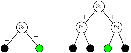
Consider the following CNF formula:

\[\Gamma_\mathrm{DPLL} := (p_1 \lor p_2 \lor \lnot p_3) \land (\lnot p_1 \lor p_2 \lor p_3) \land (\lnot p_1 \lor \lnot p_2 \lor p_3) \land (p_1 \lor p_3) \land (\lnot p_1 \lor \lnot p_3)\]

Selecting \(p_3\) as decision variable in the root node results in a DPLL tree with two leaf nodes. However, when selecting \(p_2\) as decision variable in the root node, the DPLL tree consists of four leaf nodes. The figure below shows the DPLL trees with green nodes denoting satisfying assignments, while black nodes denote falsifying assignments.

We have implemented a basic version of the DPLL procedure in Lean, which can be found in the Examples folder. We will start at the top level and work our way down. The function dpllSat accepts a CNF formula and returns either a satisfying assignment or none if there aren’t any. It calls propagateUnits to perform unit propagation, and then calls dpllSatAux to iteratively pick an unassigned variable and split on that variable. We use the keyword partial to allow for an arbitrary recursive call.

partial def dpllSatAux (τ : PropAssignment) (φ : CnfForm) :
    Option (PropAssignment × CnfForm) :=
  if φ.hasEmpty then none
  else match pickSplit? φ with
  -- No variables left to split on, we found a solution.
  | none => some (τ, φ)
  -- Split on `x`.
  -- `<|>` is the "or else" operator, which tries one action and if that fails
  -- tries the other.
  | some x => goWithNew x τ φ <|> goWithNew (-x) τ φ

where
  /-- Assigns `x` to true and continues out DPLL. -/
  goWithNew (x : Lit) (τ : PropAssignment) (φ : CnfForm) :
      Option (PropAssignment × CnfForm) :=
    let (τ', φ') := propagateWithNew x τ φ
    dpllSatAux τ' φ'

/-- Solve `φ` using DPLL. Return a satisfying assignment if found, otherwise `none`. -/
def dpllSat (φ : CnfForm) : Option PropAssignment :=
  let ⟨τ, φ⟩ := propagateUnits [] φ
  (dpllSatAux τ φ).map fun ⟨τ, _⟩ => τ

The function pickSplit? naively chooses the first variable it finds. It follows the Lean convention of using a question mark for a function that returns an element of an option type.

def pickSplit? : CnfForm → Option Lit
  | []       => none
  | c :: cs  => match c with
    | x :: _ => x
    | _      => pickSplit? cs

The function propagateUnits performs unit propagation and returns the resulting formula and the augmented truth assignment. As long as there is a unit clause, it simplifies the formula and adds the new literal to the assignment.

partial def propagateUnits (τ : PropAssignment) (φ : CnfForm) : PropAssignment × CnfForm :=
  -- If `φ` is unsat, we're done.
  if φ.hasEmpty then ⟨τ, φ⟩
  else match φ.findUnit with
    -- If there are no unit clauses, we're done.
    | none   => ⟨τ, φ⟩
    | some x =>
      -- If there is a unit clause `x`, simplify the formula
      -- assuming `x` is true and continue propagating.
      let φ' := simplify x φ
      if τ.mem x.name
      then panic! s!"'{x}' has already been assigned and should not appear in the formula."
      else propagateUnits (τ.withLit x) φ'

The function propagateWithNew is used to perform a split on the literal x. It assigns the value of x and then does unit propagation.

def propagateWithNew (x : Lit) (τ : PropAssignment) (φ : CnfForm) :
    PropAssignment × CnfForm :=
  propagateUnits (τ.withLit x) (simplify x φ)

Finally, the function simplify simplifies a CNF formula by assigning the literal x to true, assuming x is not one of the constants ⊥ or ⊤.

def simplify (x : Lit) (φ : CnfForm) : CnfForm :=
  assert! x != lit!{⊥} && x != lit!{⊤}
  match φ with
  | []      => []
  | c :: cs =>
               let cs' := simplify x cs
               -- If clause became satisfied, erase it from the CNF
               if c.elem x then cs'
               -- Otherwise erase any falsified literals
               else c.eraseAll x.negate :: cs'

#eval toString <| simplify lit!{p} cnf!{p -q p -p, p, q q, -q -p, -p}

6.4. Autarkies and 2-SAT

Unit propagation and the pure literal rule form the core of the DPLL algorithm. In this section, we present a generalization of the pure literal rule, and we illustrate its use by providing an efficient algorithm for a restricted version of SAT.

The notion of an autarky or autarky assignment is a generalization of the notion of a pure literal. An autarky for a set of clauses is an assignment that satisfies all the clauses that are touched by the assignment, in other words, all the clauses that have at least one literal assigned. A satisfying assignment of a set of clauses is one example of an autarky. The assignment given by the pure literal rule is another. There are often more interesting autarkies that are somewhere in between the two.

Notice that if \(\tau\) is an autarky for \(\Gamma\), then \(\tval{\Gamma}_\tau \subseteq \Gamma\). To see this, suppose \(C\) is any clause in \(\Gamma\). If \(C\) is touched by \(\tau\), then \(\tval{C}_\tau = \top\), and so it is removed from \(\tval{\Gamma}_\tau\). If \(C\) is not touched by \(\tau\), then \(\tval{C}_\tau = C\). Since every element of \(\tval{\Gamma}_\tau\) is of one of these two forms, we have that \(\tval{\Gamma}_\tau \subseteq \Gamma\).

Theorem

Let \(\tau\) be an autarky for formula \(\Gamma\). Then \(\Gamma\) and \(\tval{\Gamma}_\tau\) are satisfiability equivalent.

Proof

If \(\Gamma\) is satisfiable, then since \(\tval{\Gamma}_\tau \subseteq \Gamma\), we know that \(\tval{\Gamma}_\tau\) is satisfiable as well. Conversely, suppose \(\tval{\Gamma}_\tau\) is satisfiable and let \(\tau_1\) be an assignment that satisfies \(\tval{\Gamma}_\tau\). We can assume that \(\tau_1\) only assigns values to the variables of \(\tval{\Gamma}_\tau\), which are distinct from the variables of \(\tau\). Then the assignment \(\tau_2\) which is the union of \(\tau\) and \(\tau_1\) satisfies \(\Gamma\).

We now turn to a restricted version of SAT. A CNF formula is called \(k\)-SAT if the length of all clauses is at most \(k\). 2-SAT formulas can be solved in polynomial time, while \(k\)-SAT is NP-complete for \(k \geq 3\). A simple, efficient decision procedure for 2-SAT uses only unit propagation and autarky reasoning. The decision procedure is based on the following observation. Given a 2-SAT formula \(\Gamma\) that contains a propositional variable \(p\), unit propagation on \(\Gamma\) using \(\tau(p) = \top\) has two possible outcomes: (1) it results in a conflict, meaning that all satisfying assignments of \(\Gamma\) have to assign \(p\) to \(\bot\), or (2) unit propagation does not result in a conflict, in which case the extended assignment after unit propagation is an autarky. To understand the latter case, note that assigning a literal in any clause of length two either satisfies the clause (if the literal is true) or reduces it to a unit clause (if the literal is false). So if there isn’t a conflict, then it is impossible that unit propagation will produce a clause that is touched but not satisfied.

The decision procedure works as follows. Given a 2-SAT formula \(\Gamma\), we pick a propositional variable \(p\) occurring in \(\Gamma\) and compute the result of unit propagation on \(\Gamma\) using \(\tau(p) = \top\). If unit propagation does not result in a conflict, let \(\tau'\) be the extended assignment and we continue with \(\tval{\Gamma}_{\tau'}\). Otherwise let \(\tau''(p) = \bot\) and we continue with \(\tval{\Gamma}_{\tau''}\). This process is repeated until the formula is empty, which indicates that the original formula is satisfiable, or contains the empty clause, which indicates that the original clause is unsatisfiable.

6.5. CDCL

The Conflict-Driven Clause-Learning (CDCL) decision procedure is the most successful SAT solving paradigm. Although it evolved from DPLL, modern implementations of CDCL have hardly any resemblance with the classic decision procedure. The algorithms differ in core algorithmic choices. When designing an algorithm, one typically needs to choose between making the algorithm smart or making it fast. Having it both ways is generally not an option due to conflicting requirements for the datastructures. State-of-the-art DPLL algorithms are designed to be smart: spend serious computational effort to pick the best variable in each recursive call to make the binary tree relatively small. As we will describe below, CDCL focuses on being fast. Unit propagation is by far the most computationally expensive step and everything in a CDCL solver is designed by make that as fast as possible. That prevents more complicated heuristics. Another important design decision for SAT solving algorithms is determining whether you plan to find a satisfying assignment or prove that none exists. DPLL focuses on finding a satisfying assignment by picking the most satisfiable branch first, while CDCL, as the name suggests, prefers conflicts and wants to find a short refutation. A satisfying assignment is a counterexample to the claim that no refutation exists.

The early development of CDCL is four decades later than DPLL. While DPLL simply backtracks when a conflict (leaf node) is reached, CDCL turns this conflict into a conflict clause that is added to the formula. The first and arguably most important step towards CDCL is the invention which clause to add: the first unique implication point. The first unique implication point is an invention by Marques-Silva and Sakallah (1996) and is still used in all modern day top-tier solvers.

The best decision heuristic for CDCL selects the unassigned variable that occurs most frequently in recently learned conflict clauses. This heuristic, called Variable-State Independent Decaying Sum (VSIDS in short), was introduced in the zChaff SAT solver by Moskewicz and co-authors (2001). The heuristic was been improved over the years, in particular by Eén and Sörensson (2003) in their solver MiniSAT. In recent years some other advances have been made as well. However, selecting variables in recent conflict clauses is still the foundation.

Adding clauses to the input formula could significantly increase the cost of unit propagation. Therefore clause learning was not immediately successful. The contribution that showed the effectiveness of clause learning in practice is the 2-literal watchpointers datastructure. In short, the solver does not maintain a full occurrence list of clauses, but only an occurrence list of the first two literals in a clause. These first two literals are required to have the following invariant: either both literals are unassigned or one of them is assigned to true. That invariant is enough to ensure that the clause is not unit. In case an assignment breaks the invariant, then the entire clause is explored to check whether it is possible to fix the invariant by swapping a satisfied or unassigned literal to the first two positions. If this is not possible, the clause is unit and the unassigned literal is assigned to true or the clause is falsified which triggers the learning procedure in the solver.

Another key difference between CDCL and DPLL is that the former restarts very frequently. Restarting sounds drastic, but simply means that all variables are unassigned. The remainder of the solver state, such as the heuristics and the learned clauses, are not altered. Modern SAT solver restart often, roughly a thousand times per second (although this depends on the size of the formula). As a consequence, no binary search tree is constructed. Instead, CDCL might be best viewed a conflict-clause generator without any systematic search.

The are various other parts in CDCL solvers that are important for fast performance but that are beyond the scope of this course. For example, CDCL solvers do not only learn many clauses, but they also aggressively delete them to reduce the impact on unit propagation. Also, CDCL solvers use techniques to rewrite the formula, so called inprocessing techniques. In top-tier solvers, about half the runtime can be devoted to such techniques.

6.6. Exercises

1. Write, in Lean, a predicate isAutarky that takes an assignment \(\tau\) (of type PropAssignment) and a CNF formula \(\Gamma\) (of type CnfForm) and returns true or false depending on whether \(\tau\) is an autarky for \(\Gamma\).

2. Write in Lean a function getPure that takes a CNF formula \(\Gamma\) and returns a List Lit of all pure literals in \(\Gamma\). The function does not need to find all pure literals on pure literal assignment until fixpoint, only the literals the are pure in \(\Gamma\).